Exercise 1 of Tensor Flow tutorial is building one-layered neural network with softmax normalization of the outputs. It achieves 92% accuracy in recognition. Exercise 2 is training small convolutional neural network. First convolutional layer contains 32 5x5 features, is max-pooled and connected to second convolutional layer with 64 features, which is then processed by a densely connected layer. Final accuracy raises from 92% to approximately 99%.
When thinking about how neural network operates, I realized that the handwritten images are only a small subset of images that network can classify as “digits”. Network have 10 outputs, each output corresponds to a specific digit. Pixels intensities are fed to 28x28 = 784 input neurons, are processed by a network so that and each output holds a number from 0 to 1, which roughly translates as how sure network is that input was a corresponding digit.
Network is uncertain about random images, and maximal values in output layer rarely exceed 0.6. On the other hand, network is usually pretty sure about the answer when presented with MNIST examples: maximal values in output layer are typically greater than 0.9, and often are very close to 1.
So, I wondered, what other images would be recognized by a convoluted network as digits with certainty close to 1. This is like making identikits of handwritten numbers by asking network a question. First, I took a blank base image, generated 500 random masks where pixels were randomly perturbed, and added masks to a blank base to obtain perturbed image candidates. Then I run neural network, and ask it what candidate has maximal likeness to a specific digit by checking its output channel. The best image is kept and used as a base for the next iteration – until network is absolutely sure that what it perceives is an image of a digit.
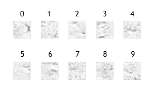
I repeated this process several times for all digits. Here is what I’ve got:
Some basic observations:
- The process of image generation is random, but most of the time resulting images have similarity within each class, and some easily recognizeable features that distinguish a class from other classes.
- One can easily see 0 and 6 in computer-generated images of zero and six. However, it take some imagination to see 3 in F-like generated shapes or 4 in u-like shapes. 1 and 9 look like a total mess.
- Sometimes network got stuck in local minima and none of the generated noisy images could improve recognition of the base image above a certain level. But in most cases confidence raised to 0.99 and above easily. 7 and 9 were the most difficult images to articulate – network converged to 0.99 in 30% of “9” cases and in 50% of “7” cases.
So, when all traces of human civilization will be gone except for the last handwritten digits recognition neural network, the aliens archeologists could make a reconstruction of how we wrote digits:


