Reverse image recognition

Recently I started exploring Tensor Flow, a wonderful library for machine intelligence, released by Google. As tutorial put it, the “Hello World” of machine learning is recognition of handwritten digits. There is a standard database containing 60,000 images and corresponding labels, it is called MNIST.

Exercise 1 of Tensor Flow tutorial is building one-layered neural network with softmax normalization of the outputs. It achieves 92% accuracy in recognition. Exercise 2 is training small convolutional neural network. First convolutional layer contains 32 5x5 features, is max-pooled and connected to second convolutional layer with 64 features, which is then processed by a densely connected layer. Final accuracy raises from 92% to approximately 99%.

When thinking about how neural network operates, I realized that the handwritten images are only a small subset of images that network can classify as “digits”. Network have 10 outputs, each output corresponds to a specific digit. Pixels intensities are fed to 28x28 = 784 input neurons, are processed by a network so that and each output holds a number from 0 to 1, which roughly translates as how sure network is that input was a corresponding digit.

Network is uncertain about random images, and maximal values in output layer rarely exceed 0.6. On the other hand, network is usually pretty sure about the answer when presented with MNIST examples: maximal values in output layer are typically greater than 0.9, and often are very close to 1.

So, I wondered, what other images would be recognized by a convoluted network as digits with certainty close to 1. This is like making identikits of handwritten numbers by asking network a question. First, I took a blank base image, generated 500 random masks where pixels were randomly perturbed, and added masks to a blank base to obtain perturbed image candidates. Then I run neural network, and ask it what candidate has maximal likeness to a specific digit by checking its output channel. The best image is kept and used as a base for the next iteration – until network is absolutely sure that what it perceives is an image of a digit.

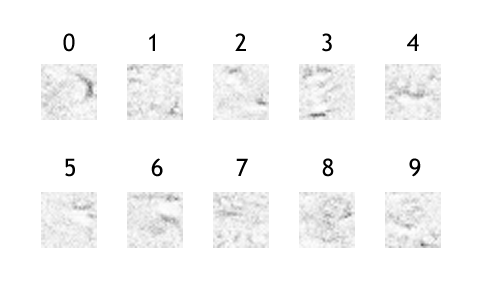
I repeated this process several times for all digits. Here is what I’ve got:

Some basic observations:

• The process of image generation is random, but most of the time resulting images have similarity within each class, and some easily recognizeable features that distinguish a class from other classes.
• One can easily see 0 and 6 in computer-generated images of zero and six. However, it take some imagination to see 3 in F-like generated shapes or 4 in u-like shapes. 1 and 9 look like a total mess.
• Sometimes network got stuck in local minima and none of the generated noisy images could improve recognition of the base image above a certain level. But in most cases confidence raised to 0.99 and above easily. 7 and 9 were the most difficult images to articulate – network converged to 0.99 in 30% of “9” cases and in 50% of “7” cases.

So, when all traces of human civilization will be gone except for the last handwritten digits recognition neural network, the aliens archeologists could make a reconstruction of how we wrote digits:

A border and a twist

One of the things that inevitably pop-up in any simulation is limit on available computational power. In particular case of simulating 2D lattice model there are 2 general ways to cope with these limitations. The first and the most straightforward thing to do is to make border of the lattice “special” in some way. For example, cells in the bulk might have 8 neighbors, cells on the border have 5 neighbors, and cells in the corners have only 3 neighbors. Usually, this means that behaviour of the system changes on the border, but when done right this does not lead to any catastrophic failure during the simulation. Here is an example of what I've got after simulating a small grid with borders:

Second way to cope with limited computational resources is to make use of periodic boundary conditions. The simplest case of periodic boundary conditions are those of asteroid game, where adjacent screens wrap on each other, and shells fired at the right edge of the screen appear at the left edge:

The overall shape of the simulation field is a torus, or more precisely, a flat torus:

But there are more twisted ways to stich the simulation fields together than just tile screens next to each other. Imagine I would take the top, twist it and glue to the bottom.

There may be even more twists to the way how ends of the screen are glued together. Here is the general blueprint of how it would look:

The overall pattern of Ising model would be different. In chaotic model these changes would be imperceptible, but when the temperature is low, the pattern would acquire certain features to it. Here how these features manifest themselves when field is annealed a number of times:

Regular patterns have a certain degree of rectangularity to them, while twisted patterns are more diagonal-like. Situations where top and bottom have opposite colors can only happen in a doubly twisted simulations.

Color perception and antiferromagnetism

Here’s another thing about color chaos aka unitary vector field that makes it different from an Ising model: the energy function can be screwed up.

I’ve implemented the way of skewing it. Cell see its neighbors through light filter. In red area, it thinks its neighbors are slightly bluer than itself, whereas in reality they have the same color. In the similar fashion the blue cells are seen slightly greener, and green cells – slightly redder. This gives interesting psychedelic effects with variation of colors.

Interestingly, the rate at which colors changed depended on temperature – at high temperatures the changes were more rapid. That would be fun to explore in details how areas with different temperatures will interact with each other.

I could change color perception a little, but nothing stops me from making more radical change. For example, I could force cells see in inverted colors: cyan instead of red, magenta instead of green and yellow instead of blue. What I will get is model of antiferromagnetism.

Antiferromagnetic ordering

In antiferromagnets spins (little magnets) try not to be aligned with each other, but to have opposite orientations. Here is what YouTube made of a video of what I saw when I took a random pattern, then heat it and cool down again:

New rules give new structure. Here are snapshots:

To the right is the same frame with 2 times magnifications. There were stripped pattern in Ising model (which you can explore in my app), and here it appears again, only in color.

P.S. What did compression algorithm did to the picture?

Not so random colors

When I coded colorful chaos (field of unit vectors, I think, is proper name of what it is), I stumbled on a question how to generate random colors. With Ising model there’s the only way: I have to just flip between 0 and 1, black and white. With colors I could think of two ways: I can change color to any other random color on a wheel, or I could change color to nearby color.

In principle results should be the same: if new color is widely distributed, then cells update just won’t happen very often at low temperatures, and would happen much more frequently at high temperature. Even if new color is contained to vicinity of the old color of the cell, at high temperatures it won’t depend on its neighbors and would drift to randomness very soon.

I sought to check it, and implemented two schemes. In the first version, cell can change its color randomly to any other color. This is the video of annealing (starting from completely random pattern and high temperature and slowly lowering the temperature):

In the second way new color is normally distributed around old color and half-width of distribution 0.05 radians (2.8 degrees). This is very narrow distribution, and see what happened:

See how in the first video there is a violent mixing of colors at the beginning, and then it all pass through some critical point, and stabilize. In the second video I was unable to see any critical temperature. The system is cooled extremely smoothly.

I started experimenting with new way of generating colors, and found out that at high temperatures it behaves quite unexpectedly. The noise at high temperatures looked completely different. When I started from the field of red and raised temperature to high values, this is what I get:

Would I run the same simulation with the first way of generating colors, it would be complete mess almost instantly. But here – it preserved structure no matter how long I waited.

Colorful chaol

Soon after I made first version of Visual Chaos app, I started to think about something even more psychedelic than Ising model. What if instead of black and white there were colors? Say, each cell will have a color, and it likes to be surrounded by the cells of the same color.

The simplest way to do it that I thought of is to make use of color wheel:

If colors of two cells are near each other on the wheel, then their energy is minimal. If colors are opposite, energy is at its maximum.

Just as in regular Ising model, from time to time the cell will try to change its color. If cell is cool, it will change to minimize its energy, if cell is hot it may change even if energy goes up. Here is what I got. In the simulation the temperature first goes up, then down again to near zero.

If you see, at the last frame there are some interesting features – little color wheel, points where all colors meet each other, like on the color wheel. Little color wheels cannot be optimized out by lowering temperatures. If you think of it, it’s a deadlock configuration: take red cell, it has orange and magenta neighbors. If it moves to orange, magenta neighbor will object, if it moves to magenta, orange neighbor will be unhappy. The problem cannot be solved by small incremental steps; the only way to solve it is to heat it up, disrupt all colors, then cool down and see if it’s ok. I’ll call such points poles.

Another funny thing about poles is that they come into pairs. Here are few examples of annealing results:

There are poles that go from red to green to blue in clockwise direction, and there are poles that go in counter-clockwise direction. From time to time clockwise and counter-clockwise points collapse and annihilate, for example in this video:

I bet there are a some rules to be learned about how many poles can be formed, and how they evolve over time.

How Ising model works

Although there is a description of an Ising model at Wikipedia, I guess it would scare a lot of people, so here is my brief explanation of how it works.

The simplest way to understand Ising model is to imagine chessboard. In a rectangular 8-by-8 grid there are 64 black or white cells. These cells are able to change their color from time to time: there is a chance that black cell become white, and white cells become black. Probability of color flip for each cell depends on its neighborhood. The general rule of Ising model is that cells likes to be surrounded by cells of the same color. If there is single white cell, surrounded by 8 black ones, it will flip its color almost instantly. On the other hand, if a white cell has 8 white neighbors, the probability that it will turn black is much lower.

What makes Ising model so interesting is temperature. The temperature sets minimal level of noise in the system. At low temperature there is almost no chance that cell surrounded by the cells of the same color will suddenly change its color. When temperature is raised this chance also rises, and at some point cell start to change its color randomly and independently of its neighbors.

This simple model already displays profound properties, related to phase transitions. If temperature is low, cells of the same color tend to cluster together, merge into larger areas until the whole grid will have uniform color. As temperature goes up, the tendency to cluster together gives way to a noise. When temperature crosses critical value, the pattern of large areas breaks, and system transits to its chaotic state.

Evolution of the system from hot chaotic state (left) to cold ordered state (right)

The bigger the system, the sharper is transition between chaotic and ordered states. To avoid uncertainty with cells on the borders, periodic boundaries are usually used: cells from the leftmost column interact with cells from the rightmost column, and cells from the top raw interact with cells from the bottom raw as if the grid is spread on the surface of the torus.

Simulation of Ising model with temperature bouncing around critical point